Datasheet and application notes for the Speake & Co FGM-1, FGM-2 and FGM-3 fluxgate-type magnetic field sensors. FGM-Series Magnetic Field Sensors
Key Features
- +5 volt single-supply operation
- Simple three-terminal devices
- DC to 20 kHz bandwidth
- Low temperature sensitivity
- High intrinsic sensitivity
- Built-in feedback coils
Description
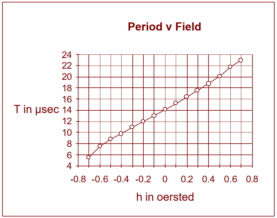
The FGM-series are very high sensitivity magnetic field sensors that operate over a ±50 microtesla range (±0.5 oersted). They’re simple three-terminal devices running from a single +5 volt supply, with connections for ground, +5V and output. The output is a robust 5 volt rectangular pulse whose period is directly proportional to field strength — in other words, the output frequency varies inversely with the field — which makes the sensor easy to interface directly to a computer or microcontroller. For the FGM-3, the period sweeps from about 8.5 µs to 25 µs (roughly 120 kHz down to 50 kHz) across the full range, illustrating just how sensitive the device is.
The FGM-1 is essentially a miniature version of the FGM-3 with slightly lower sensitivity. The FGM-2 packages two FGM-1 sensors at right angles to each other in a single housing.
Unlike Hall-effect sensors — which are largely unusable in this range due to high temperature sensitivity — the FGM-series has a very low temperature coefficient. Because the lowest effective Nyquist sampling rate is around 50 kHz, appropriate filtering can deliver an AC field bandwidth from DC up to roughly 20 kHz.
Electrical Specifications
| Parameter | Value |
|---|---|
| Maximum Supply Voltage | 7 volts |
| Recommended Supply Voltage | 5 volts ± 0.5 volts |
| Typical Supply Current | 12 mA |
| Operating Temperature Range | 0 – 50 °C |
Typical Applications
Because the sensor’s range covers the magnitude of the earth’s field, multiple sensors can easily be arranged for compass orientation or full three-dimensional orientation systems — gimballed compasses, virtual-reality helmet tracking, and similar uses that reference the local earth field.
Other applications include conventional and earth-field magnetometry, ferrous metal detection, internal vehicle re-orientation alarms, external vehicle or ship passage sensors, wreck-finding, non-contact current sensing, conveyor belt counters, and — paired with small permanent magnets — movement/proximity sensing and ferrous-impurity detection in non-magnetic alloys.
Conventional magnetometry applications include magnetic material measurement, B-H loop measurement, Preisach displays and archaeological artifact assessment.
For applications needing a wider field range, external feedback-winding techniques can extend both maximum range and linearity: an overwound solenoidal coil is placed in a negative feedback loop that continuously drives the field seen by the sensor toward zero, so range and linearity become a function of the feedback coil current rather than the raw sensor characteristics. The miniature FGM-1 and FGM-2 have such a coil built in for convenience.
Typical Characteristics
The chart below shows the typical Period vs. Field response of the larger sensor, the FGM-3. Between ±0.5 oersted (±50 µT), non-linearity is about 5.5%.
Period vs Field chart for FGM-3 sensor
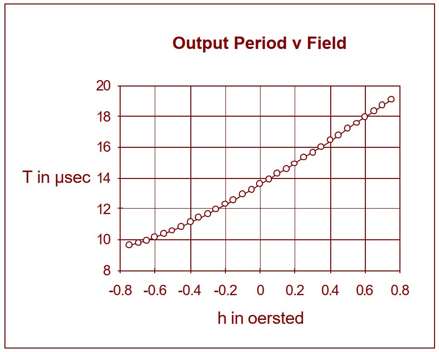
The miniature sensors (FGM-1 and FGM-2) show a similar curve, with non-linearity of about 4.8% across the same ±0.5 oersted range. This non-linearity varies somewhat between individual sensors but is normally around 5%.
Improving Linearity
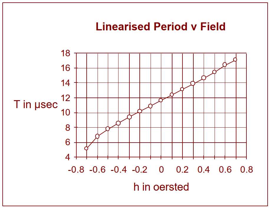
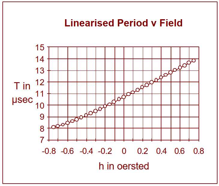
Field strength is not simply inversely proportional to frequency — in practice it’s more closely inversely proportional to frequency plus a small constant. If a fixed number of kilohertz is added to the measured frequency before inverting it to get the period, the period-vs-field curve becomes much more linear.
Adding a fixed 15 kHz to the FGM-3’s incoming frequency before inversion (T = 1/(f + c), c = 15 kHz) reduces non-linearity between ±0.5 oersted from 5.5% down to just 0.7%.
Period vs Field chart for FGM-1 and FGM-2 sensors
The same trick works for the miniature sensors, typically with a constant of about 18 kHz.
For FGM-1/FGM-2, the built-in overwound coil can additionally be used as a simple biasing coil — injecting roughly −1 mA into the feedback pin (e.g. via a 4.7 kΩ resistor to a −5 volt supply) shifts the zero-field point and further improves linearity, reducing non-linearity from 4.8% to 0.2% across an increased range of ±0.7 oersted.
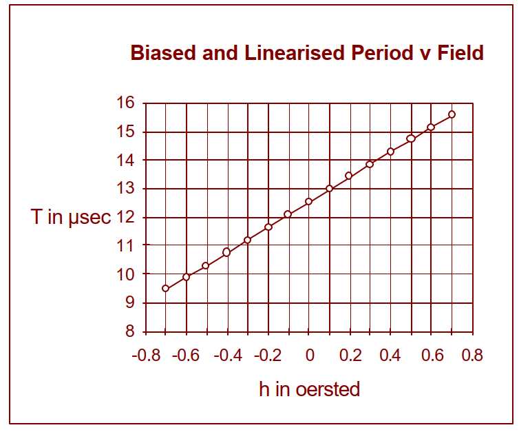
Biased and Linearised Period v Field — FGM-1 / FGM-2
If period is measured directly rather than frequency, the same linearising approach still applies: use T/(T + cT) as the quantity proportional to field strength, where T is in microseconds and c is in kilohertz.
Supply Voltage Sensitivity
Output period varies with supply voltage at roughly 3.5% per volt around the nominal 5 volt level. Precise applications need good supply regulation — but since current draw is low, this is easy to achieve with simple regulators such as the LM78L05 series.
General Application Notes
Use with Computers and Microcontrollers
The large pulse output gives good noise immunity, allowing sensors to be sited at long distances from the main system. Interfacing needs just one digital input bit per channel: count pulses over a fixed period to get frequency, or measure the time between successive edges for a faster, direct period reading. Most microcontrollers handle this easily; heavily interrupt-driven or multitasking systems may need input buffering — typically just a triple-counter I/O chip, even for a three-axis system.
For long-interval readings (e.g. earth-field magnetometry), a simple binary divider chip reduces the input period to a manageable rate. Where field variation is very small, digital heterodyning against a stable oscillator reduces the period while preserving high sensitivity (in Hz/oersted).
Absolute field magnitude without orientation sensitivity requires three orthogonal sensors, exploiting the fact that the sum of the squares of the three signals is constant regardless of orientation — provided zero offsets, channel sensitivities and linearisation are properly calibrated.
Physical Characteristics — Sensor Outline (FGM-3)
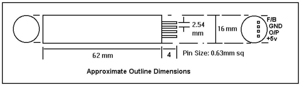
FGM-3 sensor outline dimensions
The sensor’s cylindrical form makes it easy to overwind with external feedback coils, or to insert into a separately fabricated coil on a tubular core. As a rule of thumb, a single layer of 0.2 mm wire wound over 60 mm of sensor length gives roughly 4000 turns/metre. Since 1 oersted ≈ 80 ampere-turns/metre, such a winding produces about 50 oersted per ampere — so up to 100 mA can offset fields of ±5 oersted, extending sensor range by roughly 10×, while negative feedback also improves linearity and stability.
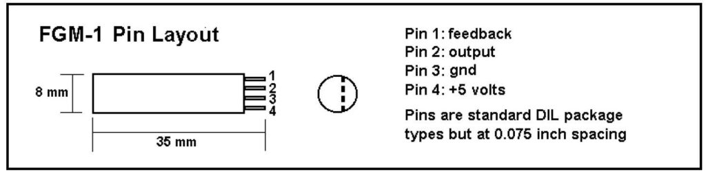
FGM-1 pin layout diagram, 35mm x 8mm package
FGM-1 Pin Layout
Pin 1: feedback | Pin 2: output | Pin 3: gnd | Pin 4: +5 volts. Standard DIL package pins, but at 0.075″ spacing.
FGM-2 Pin Layout
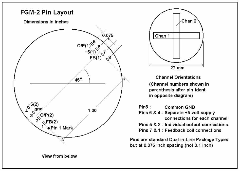
FGM-2 dual-channel pin layout diagram, 27mm package
Pin 3 is a common ground. Pins 6 & 4 give separate +5V supply connections for each channel; pins 5 & 2 are the individual output connections; pins 7 & 1 are the feedback coil connections. Standard DIL package pins at 0.075″ (not 0.1″) spacing, with the two internal sensing channels oriented at right angles to each other.
Conversion Tables
Magnetic Flux Density
| gauss | tesla | gamma | |
|---|---|---|---|
| 1 gauss | 1 | 10-4 | 105 |
| 1 tesla | 104 | 1 | 109 |
| 1 gamma | 10-5 | 10-9 | 1 |
Magnetic Field Strength
| amp/metre | oersted | |
|---|---|---|
| 1 amp/metre | 1 | 0.01257 |
| 1 oersted | 79.58 | 1 |
Note: technically the sensor measures flux density (gauss), but since in air the units of flux density and field strength share the same magnitude, oersted is used throughout as equivalent to gauss.
Application Notes: Circuit Design Techniques
Decoupling and Power Supply Regulation
With long lead lengths, local decoupling near the sensor is advisable — a 10 µF electrolytic capacitor works well. Because the sensor has a few percent sensitivity to supply variation, most applications need power regulation. A single fixed regulator (LM78L05 or equivalent) is adequate for orientation devices, but earth-field magnetometry or small-signal work needs supply variation reduced to the point where the sensor’s own temperature coefficient becomes the limiting factor.
Double regulation — 12–15V down to 9V, then to 5V, using an LM78L09 followed by an LM78L05 — is a low-cost solution for this.
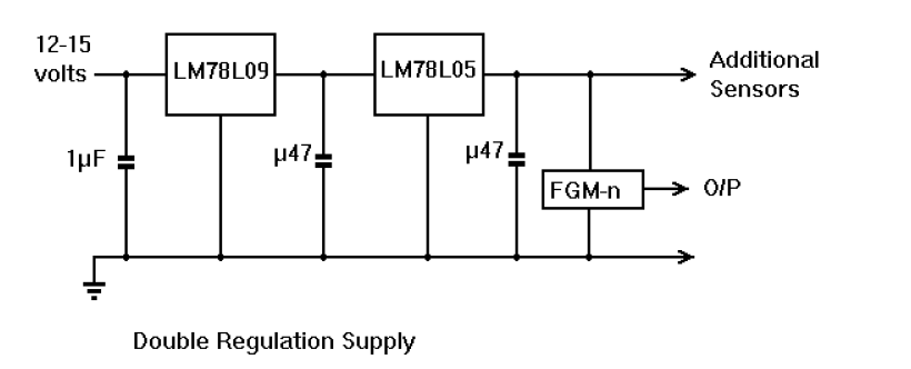
Double regulation power supply circuit diagram
Sensor Calibration
Simple field detection or orientation systems don’t need calibration. For applications that must measure field strength accurately, a close-wound single-layer solenoid on a tube (internal diameter large enough for the sensor) gives a field equal to the current times turns-per-metre — both measurable with a ruler and an ammeter. A winding at least twice the sensor’s length gives good calibration accuracy.
The field at the centre of the coil is: H = geometry-factor × turns/metre × current (H in amperes/metre).
| Length/diameter | Geometry-factor |
|---|---|
| 5 | 0.9806 |
| 6 | 0.9864 |
| 7 | 0.9900 |
| 8 | 0.9923 |
| 9 | 0.9939 |
| 10 | 0.9950 |
| Length/diameter | Reduction-factor | Uniformity |
|---|---|---|
| 5 | 0.9788 | ±1.06% |
| 6 | 0.9847 | ±0.77% |
| 7 | 0.9884 | ±0.58% |
| 8 | 0.9910 | ±0.45% |
| 9 | 0.9938 | ±0.31% |
| 10 | 0.9942 | ±0.29% |
Calibration current needs are modest — a single-layer winding of 0.5 mm enamelled wire needs only about 23 mA to reach the sensor’s full ±0.5 oersted (40 A/m) range. Align the coil and sensor perpendicular to local maximum field (e.g. east-west) during calibration; an accurate zero-field point requires a mumetal shielded enclosure, also aligned east-west.
Linearity Correction
Real-world linearity is usually better than the datasheet plots suggest, and most applications don’t need correction. Where a small concave curvature remains, it can be straightened by adding a proportion of the period-squared term to the assumed linear relationship:
H = c₀ + c₁(T − T₀) + c₂(T − Tmin)²
Measuring full-scale negative and positive periods plus the zero-field period gives three simultaneous equations to solve for c₀, c₁, and c₂. Normalising by the zero-field period (T₀ = 1):
- −0.5 = c₀ + c₁(Tmin − 1) (measured at −0.5 oersted)
- 0 = c₀ + c₂(1 − Tmin)² (T₀ = 1)
- 0.5 = c₀ + c₁(Tmax − 1) + c₂(Tmax − Tmin)² (measured at +0.5 oersted)
c₁ is the usual linear slope, c₂ is the small period-squared correction, and c₀ offsets the disturbance the squared term introduces at zero field.
Field Measurement Methods
The simplest method is a frequency meter on the sensor output, set to period mode — adequate for calibration and familiarisation, though most designs will automate the conversion.
Meter or Chart Recorder Output
A semiconductor frequency-to-voltage converter such as the LM2907 makes a low-cost, portable direct-reading instrument. Since field strength is inversely proportional to frequency, the meter scale isn’t perfectly linear, but over ±0.5 oersted the non-linearity is modest and gives an acceptably spaced scale — at higher sensitivities over a narrower range it becomes negligible. Where the converter can’t handle the highest output frequency, a binary prescaler brings it into range; a phase-locked loop is an alternative to the diode-pump converter.
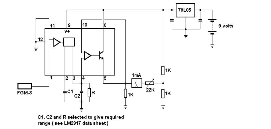
Digital Heterodyning
Where the sensor’s full range isn’t needed — ferrous detection, or measuring small field fluctuations — digital heterodyning gives very high sensitivity to small signal changes. A stable, adjustable clock close in frequency to the sensor output undersamples the sensor signal (e.g. via a D-type bistable, sensor output on D, clock on the trigger input), producing a much lower beat frequency proportional to the difference between the two.
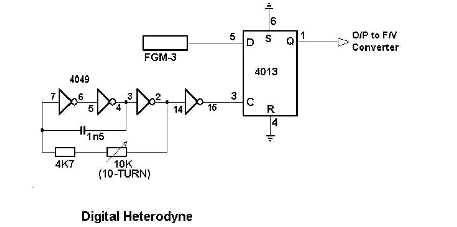
Digital heterodyne circuit using 4049 oscillator and 4013 D-type bistable
A small percentage change in sensor frequency becomes a large percentage change in the bistable output — boosting apparent sensitivity without extra gain stages. This CMOS oscillator configuration is stable enough for ferrous-metal detectors; one such arrangement reportedly detected a passing motorcycle in the far lane of a three-lane road from the grass verge. Earth-field or materials magnetometry needs a more stable (e.g. crystal) oscillator, since the fixed frequency doesn’t need to track a moving platform. The same technique applies to counting objects on a conveyor belt — remembering that field from a magnetic moment falls off as the inverse cube of distance, not the inverse square.
Earth Field Magnetometer
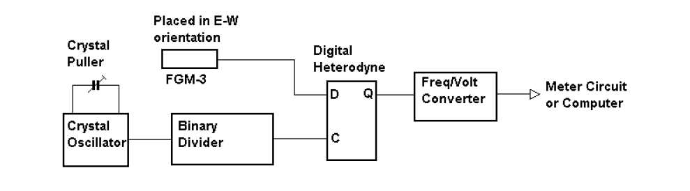
With the sensor oriented east-west, a crystal oscillator and binary divider are set to about 500 Hz below the sensor’s mean frequency and fed into the digital heterodyne circuit. The FGM-3’s sensitivity gives a swing of roughly 0–1000 Hz for a ±500 gamma field variation (1 gamma = 10⁻⁵ oersted) — enough headroom for most magnetic storm activity. The heterodyne output feeds a voltage-to-frequency converter for chart recording, or a computer for data logging; with a calibrated sensor, results convert to angular/azimuth variation by dividing by the local horizontal field component.
Such a magnetometer needs to sit well away from interference sources like transformers and vehicles — though the inverse-cube falloff helps considerably. One exception: during commissioning, a small ceramic magnet placed at a suitable distance can be used to deliberately “pull” the sensor frequency to help match it against the divider chain.
Materials Magnetometer
Materials magnetometer configuration diagram
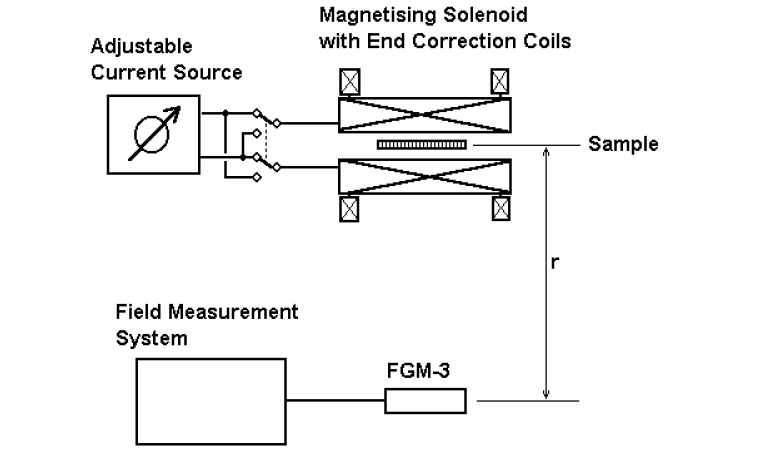
The same sensitivity supports a classical Gauss-type materials magnetometer: an adjustable-current magnetising solenoid (or electromagnet yoke, for high-susceptibility materials) alongside a field-measuring sensor. Cycling the magnetising coil through positive and negative saturation traces the sample’s hysteresis loop. To avoid shearing the loop, use a specimen with a small (or known, correctable) demagnetising coefficient, such as a cylinder — and for quantitative induction measurement, keep the sensor distance large relative to the specimen’s magnetic length.
Calibration typically uses a standard reference sample. Superimposing an AC source on the DC supply also supports anhysteretic magnetisation — something conventional AC-driven B-H loop testers can’t do, since they can’t measure static fields. Naval establishments use similar fixed or portable ranges to check ship degaussing efficiency; the flip side is that sufficiently sensitive systems can locate vessels by their magnetic anomaly. Made orientation-insensitive, such detectors can also serve as remote wreck-finders for divers.
Orientation Measurement Devices
Steer-on-Heading Compass
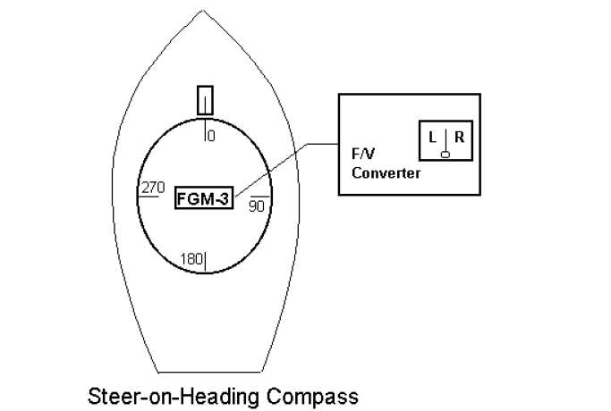
The simplest orientation device is a single-axis “steer-on-heading” compass, or poor man’s autopilot: a single sensor on a rotatable, degree-marked disk with a fixed pointer.
wp-element-caption”>Steer-on-Heading Compass
The sensor feeds a frequency-to-voltage converter driving a centre-zero meter. If the vessel veers off course, the needle deflects to indicate the correction direction and magnitude; turning the disk to a new heading shows the shortest way to steer until the new heading is reached. For this to work, the sensor must be gimballed and weighted to stay level — only a single gimbal is needed since it rotates with the heading disk.
A two-axis compass needs a microcontroller rather than a simple F/V converter, ideally one with built-in frequency or period-measurement features to match the sensor’s own analogue-to-digital nature.
Angular Sensitivity and Polar Response
An individual sensor “sees” the full field magnitude when aligned along its long axis, zero output at right angles to it, and a cosine-weighted response in between — giving the classic figure-of-eight polar diagram (two contacting circles, or spheres in 3D).
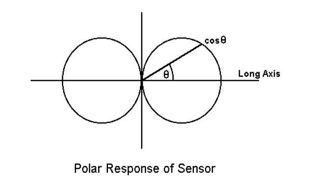
Polar response of sensor diagram
Sensors aligned along the axes of a coordinate system give outputs proportional to the direction cosines of the field vector. Readings are normalised by dividing by the zero-field period, then (for orientation devices) offset by one for equal positive/negative range. Because no two sensors have identical absolute sensitivity, a proportionality constant — from calibration-coil testing or from aligning each sensor along the local field in both directions — equalises sensitivities across the set.
Two-Axis Orientation Sensing
A two-axis compass superimposes twin sensors at right angles, both constrained to the horizontal plane. Rotating through 360° lets software auto-determine the maxima/minima needed to equalise sensitivity on both axes. Treating the standardised readings as x/y components of the field vector h (modulus √(x²+y²)), dividing each component by that modulus yields the true direction cosines — the unit vector i pointing along the field.
With the compass heading aligned to the y-axis, heading angle θ follows from tanθ = −ix/iy, i.e. θ = tan⁻¹(−ix/iy). In 3D, this extends cleanly provided the z-axis stays vertical — the necessary condition for this compass type, which needs two-axis gimballing.
Octant-Based Heading Without Trigonometry
Because a full arctangent solution isn’t ideal for low-level microcontroller code, the 360° circle can be split into eight 45° octants, identified purely from the signs of ix and iy and their relative magnitudes:
| sign of ix | sign of iy | |ix| vs |iy| | octant no. |
|---|---|---|---|
| negative | positive | less | 1 |
| negative | positive | greater | 2 |
| negative | negative | greater | 3 |
| negative | negative | less | 4 |
| positive | negative | less | 5 |
| positive | negative | greater | 6 |
| positive | positive | greater | 7 |
| positive | positive | less | 8 |
This alone gives an 8-point compass accurate to ±22.5° — adequate for undemanding applications, and its Gray-code-like structure (only one rule parameter changes at each octant boundary) avoids jitter at transitions.
Better precision comes from treating the smaller of the two direction cosines as a radian angle: with a scaling constant k = 1.08, error stays within about 1.25°; ignoring k entirely, error stays under 4.5°, enough for an easy 5°-precision compass. The general rule: whichever direction cosine is smaller is interpreted as an angle, then added to (odd octants) or subtracted from (even octants) the nearest quadrant boundary. Combined with k = 1.08, this reaches almost ±1° precision with no trigonometric functions at all — or a short lookup table of corrections can push a k=1.0 implementation to about ±0.5°:
| measured angle | added correction |
|---|---|
| 0° – 20° | 0° |
| 20° – 29° | 0.9° |
| 29° – 33° | 1.8° |
| 33° – 37° | 2.7° |
| 37° – 39° | 3.7° |
| 39° – 41° | 4.3° |
Correcting for Sensor Misalignment
A common error source is imperfect orthogonality between the two sensor axes, which produces a smoothly varying heading error that can dwarf the errors above. If φ is the small angular error in the x-axis sensor’s alignment, geometry shows the true x-component can be recovered from the apparent (measured) one by adding a small fraction of the y-component:
ix = ix′ + φ·iy
φ can be found once, either by rotating a standardised sensor set through the earth’s field and measuring the angle between each sensor’s zero-field positions, or retrospectively by averaging the heading error observed at 90° and 270° during a full rotation. The correction can then be applied in software, or read from a trimpot during a compass “boxing” procedure if the microcontroller can’t store it.
The largest real-world error usually comes from failing to keep the sensor axes horizontal — tilt errors depend on both direction and heading (a 1° east-west tilt on a north heading, for example, can produce nearly 2.5° of heading error), and the only real cures are effective double-gimballing or averaging multiple readings. A more complex option is a separate gravity sensor with trigonometric tilt correction.
Precision requirements for the raw sensor readings are surprisingly modest: 1° precision needs the measured components slotted into only 45 evenly spaced bands — about 6 bits of resolution — and 5° precision needs just 4 bits.
Three-Sensor Systems
Three orthogonal sensors give the full 3D magnitude and direction of the local field, referenced to the sensor’s own axis system rather than absolute space — useful well beyond compassing. Extending to three dimensions opens up earth-field-referenced “virtual reality” tracking with free-roving capability, though the sensor set alone is ambiguous: the axis system can rotate a full 360° around the field vector without changing the outputs. Resolving that ambiguity needs a second fixed-orientation reference — typically gravity, via an accelerometer with a flat response from DC up through the required tracking bandwidth (70–250 Hz for flicker-free VR).
Pseudo Three-Axis Systems
Some systems use a three-axis sensor set but avoid needing a gravity reference by constraining one axis mechanically instead — a searchlight, for example, rotates in azimuth and elevation but never rolls. Once the roll axis is held horizontal, the rotational ambiguity disappears and both azimuth and elevation can be solved directly. This applies to gun platforms, steerable aerials, some robotics, and potentially low-cost glider compasses: a gimballed, weighted sensor set that keeps its pitch axis roughly horizontal during steady turns could deliver a heading and bank-angle readout far better than a conventional gimballed compass, at a fraction of the cost of a gyroscopic solution.
Two- and Three-Dimensional Ferrous Detectors
A two-sensor version of the fixed vehicle detector adds angular information alongside magnitude. A passing magnetic moment’s field lines combine with the earth’s locally uniform field; a close pass produces both a magnitude swing and a large angular swing, while a remote pass produces smaller versions of both. Plotting magnitude against angle in a polar diagram gives a time-invariant “signature” for the passing object — closer passages trace a wider-angle diagram, more remote ones a narrower one (also depending on the object’s effective magnetic moment/size).
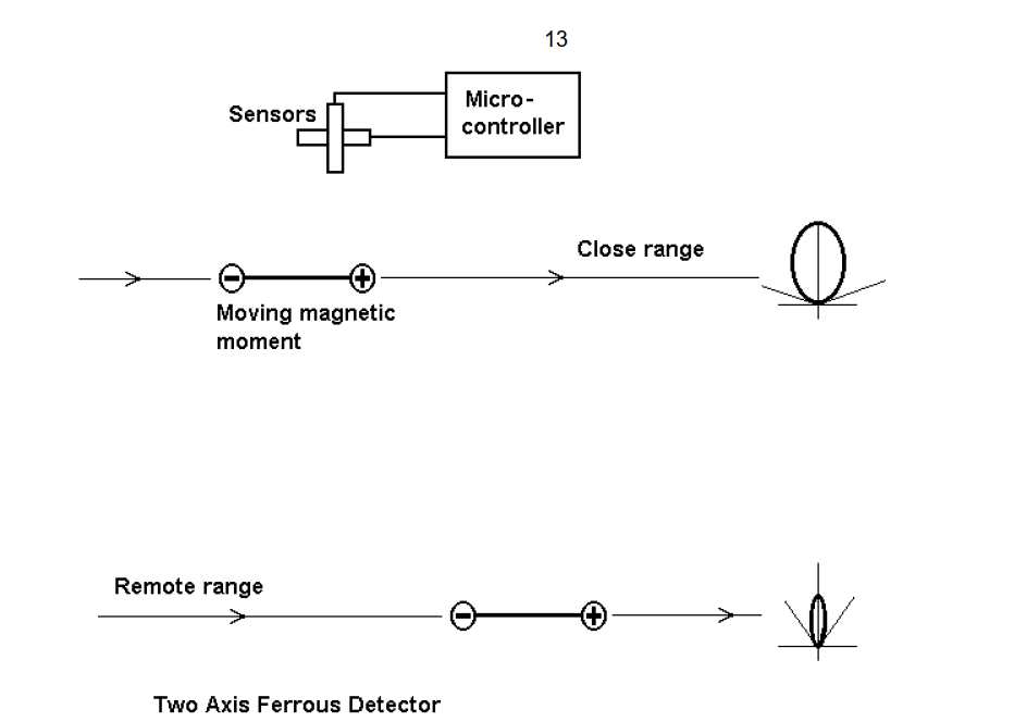
The actual variations are small but can be amplified with the digital heterodyne technique (or its software equivalent). This is a promising area for further work on lane separation and vehicle classification in traffic studies
Orientation Sensitivity Elimination
Static ferrous-detection setups can simply subtract out the earth field’s fixed contribution. But where the sensor itself moves unpredictably, high orientation sensitivity becomes a real problem. For a perfectly standardised, linearised and orthogonal sensor set, the fix is simple: the sum of the squares of the three axis outputs always equals the field vector’s modulus squared — a scalar with no orientation dependence at all. In practice, the main limiting factor is how close to “perfect” the sensor calibration actually gets.
Sensor sensitivity is generally adequate and orthogonality can be corrected fairly well, but non-linearity tends to be the most troublesome remaining error source. Negative feedback helps here too: overwinding the sensor with a solenoidal coil and driving its current to continuously cancel the local field to zero means the sensor’s own non-linearity never comes into play — the cancelling current becomes a direct, linear measure of field magnitude. With a microcontroller, this can be implemented cheaply as a single-bit PWM output through a low-pass filter, the same approach used in low-cost digital audio.
Full 360° de-sensitising isn’t always necessary — even partial reduction (e.g. a detector on a normally level vehicle, or a neutrally buoyant trailed float) can meaningfully improve stability. Built with care, this type of system can serve as a low-cost, compact detector for seabed wrecks or archaeological surveys — a practical alternative to nuclear magnetic resonance instruments in some applications.
Source: Speake & Co Llanfapley, FGM-series datasheet and application notes. Speake & Co Llanfapley, 6 Firs Road, Llanfapley, Abergavenny, Monmouthshire, NP7 8SL, UK.