DIY 3D Magnetic Imaging: Arduino Scan

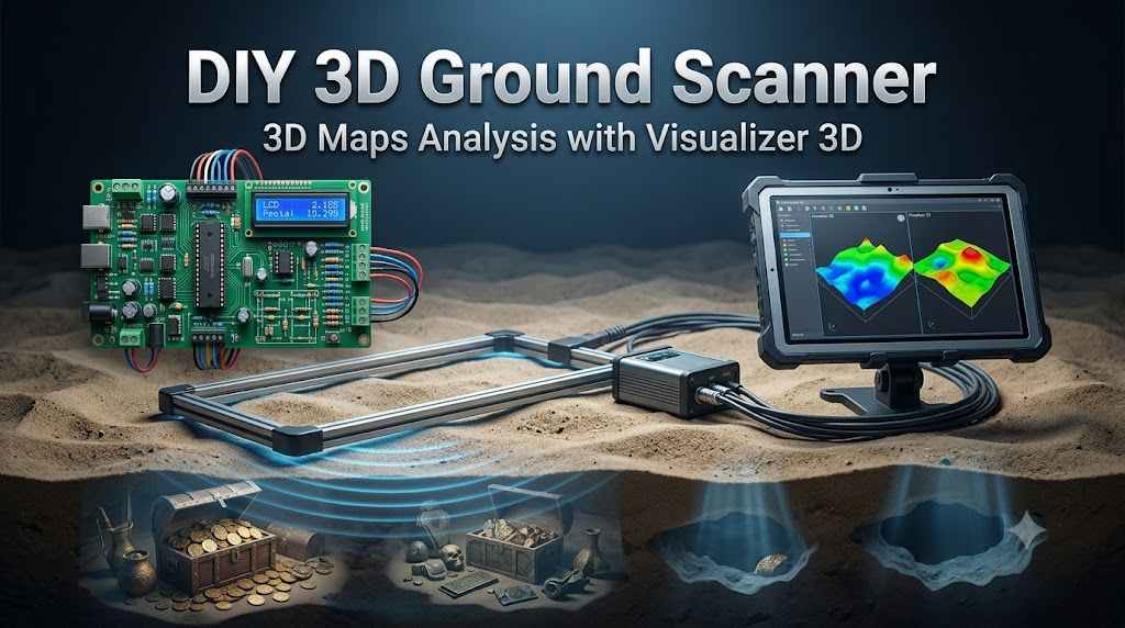
1. Project Introduction: The Geophysical Imaging

In the specialized field of subsurface exploration, the barrier to entry has historically been defined by the high cost of proprietary instrumentation. As a senior engineer in the embedded space, I view this Arduino-based magnetic scanner not merely as a hobbyist project, but as a strategic exercise in the democratization of geophysical imaging. This system bridges the gap between basic electromagnetic sensing and high-end commercial units, such as the Conrad systems, by utilizing a dual-sensor array compatible with professional-grade 3D visualization software.

The core objective of this build is to achieve high-fidelity data acquisition using remarkably accessible components; the raw materials for the sensing elements cost approximately $3 to $4, a fraction of the thousands required for commercial alternatives. This project empowers the independent researcher to visualize magnetic anomalies—ranging from structural voids to metallic deposits—with a high degree of spatial resolution. Because the 3D visualizer requires precise signal intervals and consistent data streams, the transition from hardware assembly to digital interpretation relies entirely on the integrity of our underlying system architecture.

2. System Architecture and Functional Principles

Before initiating the physical build, one must grasp the logic of differential magnetic sensing. Without a clear understanding of how the device translates environmental flux into digital packets, the resulting 3D scans will suffer from signal drift and lack the clarity required for professional analysis.

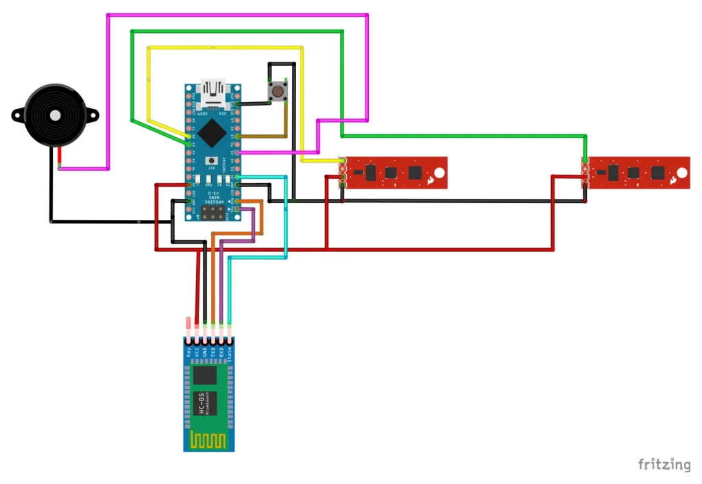
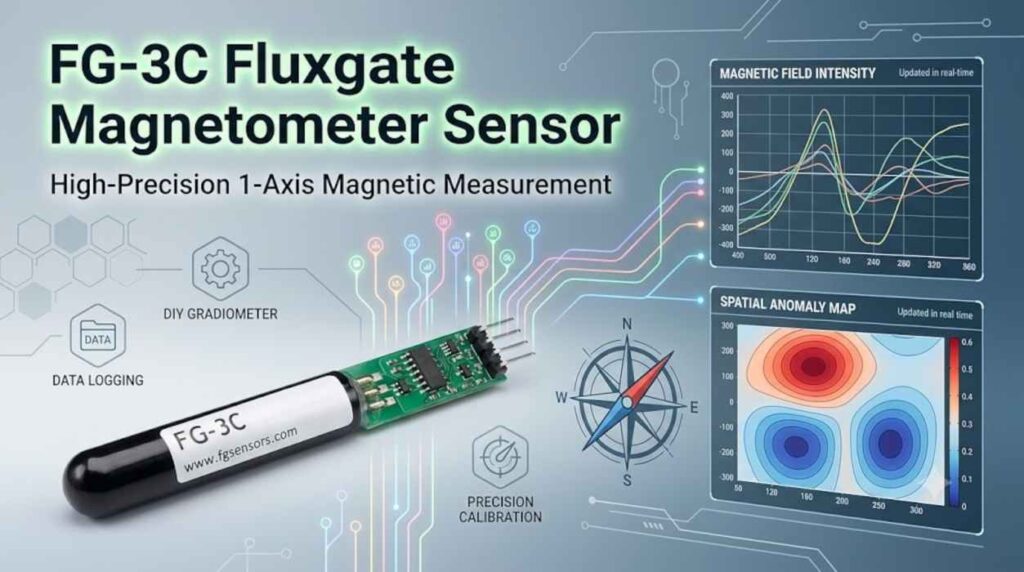
Principal Working and Signal Processing The device functions as a gradiometer, employing a dual-sensor array to detect minute electromagnetic variations. These sensors act as transducers, converting magnetic field strength into analog voltage levels. The Arduino serves as the central processing engine, utilizing its onboard Analog-to-Digital Conversion (ADC) to translate these continuous signals into discrete digital data packets. By sampling two points simultaneously, the system can begin to account for ambient magnetic noise, focusing instead on localized anomalies.

The Interpretive Role of 3D Visualization Software The 3D Visualizer software serves as the system’s interpretive engine, performing the heavy lifting of data reconstruction. Raw sensor data is essentially a unidirectional stream of intensity values; the software maps these values across a three-dimensional grid, allowing the operator to differentiate between “voids” (caves, tunnels, or soil disturbances) and “metallic objects” based on the polarity and magnitude of the magnetic response. Achieving this level of visualization depends heavily on the precision of the hardware selected for the Bill of Materials.

3. Comprehensive Bill of Materials (BOM) and Component Selection

In geophysical sensing, the resolution of your data is limited by the quality of your signal chain. Minimizing electromagnetic interference (EMI) and ensuring component reliability is critical for field readiness.

Necessary Parts List

• Microcontroller: Arduino Nano, Uno, or Mega (ATmega328P or ATmega168 variants). The ATmega328P is preferred for its superior ADC stability.
• Sensing Unit: Two custom-wound sensors utilizing thin plastic tubing (straw-diameter) and carbon-free stainless steel core ribbons.
• Communication Module: HC-05 or HC-06 Bluetooth Module.
  • Critical Setting: Default Communication Baud Rate: 9600.
• User Interface:
  • Tactile manual scan button (for localized data triggering).
  • SPST power switch.
  • Piezo buzzer (for auditory step-synchronization).
• Housing/Structure: 30cm non-metallic mounting frame (PVC or wood) to avoid interference.

The “So What?” of the Bluetooth Interface The HC-05/06 choice is pivotal for maintaining the galvanic isolation of the scanner from the workstation. While the microcontroller is flashed at high speeds, the Bluetooth link must be maintained at a default 9600 baud rate to ensure data packet integrity and stable handshaking with the 3D Visualizer software. This wireless link is what transforms a stationary bench tool into a portable field instrument, leading us directly into the most sensitive phase of the project: sensor fabrication.

4. High-Precision Sensor Fabrication

The sensor’s performance is the primary variable in the system’s signal-to-noise ratio. A meticulous tuning process is required to ensure both sensors are matched for differential sensing.

Two-Step Induction Coil Tuning

1. Initial Air-Core Winding: Wrap the copper wire around the plastic tubing using a low-RPM winding jig to ensure uniform tension. The goal is to reach a baseline inductance of 0.05 mH (50 uH) with a target resistance between 3.1 and 3.4 Ohms.
2. Core-Loading for High Inductance: To reach the required 0.8 mH (800 uH) threshold necessary for deep-field sensing, you must insert thin ribbons of carbon-free stainless steel (often sourced as specialized strapping or transformer laminations).

Calibration and Stabilization By incrementally adding or removing the steel ribbons, you can fine-tune the inductance to the exact 0.8 mH specification. Once the electrical values are matched across both sensors, the internal components must be encapsulated using wax or hot glue. This is not merely for protection; it is a strategic requirement to prevent microphonic noise and inductance instability caused by physical vibrations during the scan. With the sensors tuned for thermal and mechanical stability, we can proceed to the firmware implementation.

5. Firmware Implementation and Bluetooth Configuration

The “Hex File” defines the sampling logic and data packaging protocol. Flashing the firmware correctly is the most common failure point for DIY builds.

Software Deployment Workflow

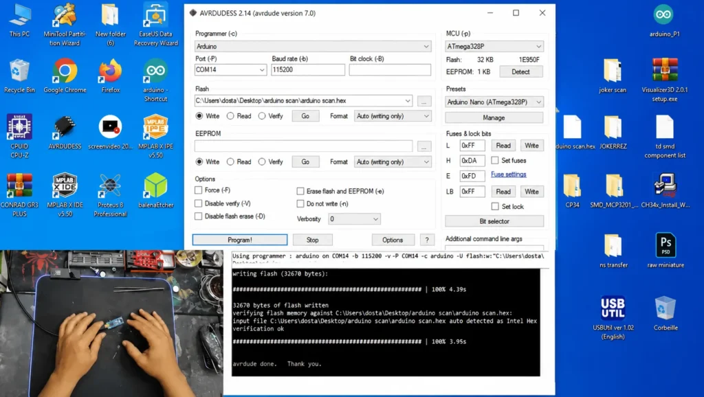
1. Tool Selection: Utilize AVRDUDE or the more user-friendly XLoader utility.
2. Configuration:
   • Select the appropriate COM port (e.g., COM14).
   • Set the Upload Baud Rate to 115200 (distinct from the 9600 communication rate).
   • Specify the target device (e.g., ATmega328).
3. The “Detect” Step: Always use the detect function first to verify the serial link to the ATmega chip before flashing.
4. Flashing: Load the .hex file and initiate the “Program” or “Upload” sequence.

Bluetooth Handshaking To ensure the 3D Visualizer recognizes the hardware, the Bluetooth module should be renamed to “ID SCAN” via AT commands. This dedicated identifier prevents the software from attempting to pair with peripheral devices, ensuring a dedicated telemetry link. Once the firmware is flashed and the wireless link is verified, the system is ready for physical integration.

6. Final Assembly and Calibration Standards

Physical geometry in a geophysical scanner is a functional requirement, not a design choice. The spatial relationship between the sensors determines the system’s ability to filter environmental clutter.

The 30cm Gradiometer Rule The two sensors must be mounted exactly 30cm apart on a rigid, non-conductive frame. From a geophysics perspective, this 30cm spatial separation establishes the baseline for the gradiometer effect. This allows the software to calculate the differential between the two points in space, effectively cancelling out the Earth’s background magnetic field and highlighting localized subsurface anomalies.

Field Synchronization Interface

• Manual Scan Button: This triggers a specific data acquisition event for the Arduino to process.
• The Buzzer “Click”: The buzzer provides auditory feedback synchronized with each button press. This ensures the researcher’s physical steps are perfectly timed with the software’s data acquisition cycle, preventing spatial distortion in the 3D render.

Final Success Checklist

• [ ] Sensors tuned to 0.8 mH and 3.1–3.4 Ohms.
• [ ] Mechanical stabilization (wax/glue) applied to coils.
• [ ] Fixed 30cm baseline separation achieved on the frame.
• [ ] Bluetooth paired as “ID SCAN” at 9600 baud.
• [ ] Buzzer “clicks” confirm successful manual triggers.

7. Conclusion: Strategic Potential of DIY Geophysical Tools

This project demonstrates that high-resolution imaging is attainable without commercial gatekeeping. By prioritizing sensor inductance and maintaining strict geometric tolerances, the DIY researcher can produce results that rival entry-level professional tools.

It is important to manage expectations regarding depth: while advanced benchmarks for this technology—utilizing secondary amplification circuits and high-gain stages—have shown capabilities reaching up to 6 meters, the basic dual-sensor build described here is optimized for high-resolution mapping of shallower subsurface targets.

Original Video

Download the Firmaware